The pipeline as a way of transporting liquid and gaseous media is the most economical way in all sectors of the national economy. This means that he will always enjoy increased attention from specialists.

Hydraulic calculation during design pipeline system allows you to determine the inner diameter of pipes and the head drop in the case of maximum pipe capacity. In this case, the presence of the following parameters is mandatory: the material from which the pipes are made, the type of pipe, productivity, physical and chemical properties of the pumped media.

Making calculations using formulas, some of the specified values \u200b\u200bcan be taken from the reference literature. FA Shevelev, professor, doctor of technical sciences has developed tables for accurate calculation of throughput. The tables contain the values \u200b\u200bof the inner diameter, resistivity, and other parameters. In addition, there is a table of approximate values \u200b\u200bof velocities for liquids, gas, water vapor to simplify the work with determining the throughput of pipes. Used in utilities where accurate data is not essential.

Calculated part

Calculation of the diameter begins with the use of the formula for uniform fluid movement (continuity equation):

where q is the estimated flow rate

v is the economic speed of the current.

ω is the cross-sectional area of \u200b\u200ba circular pipe with a diameter d.

Calculated by the formula:

where d is the inner diameter

hence d \u003d √4 * q / v * π

The speed of fluid movement in the pipeline is taken equal to 1.5-2.5 m / s. This is the value that corresponds to the optimal performance of the linear system.

The head loss (pressure) in the pressure pipeline is found using the Darcy formula:

h \u003d λ * (L / d) * (v2 / 2g),

where g is the acceleration of gravity,

L is the length of the pipe section,

v2 / 2g - parameter denoting the velocity (dynamic) head,

λ - coefficient of hydraulic resistance, depends on the mode of fluid movement and the degree of roughness of the pipe walls. Roughness means roughness, defect of the inner surface of the pipeline and is divided into absolute and relative. Absolute roughness is the height of the irregularities. The relative roughness can be calculated using the formula:

The roughness is different in shape and uneven along the length of the pipe. In this regard, the calculations are based on the average roughness k1 - a correction factor. This value depends on a number of points: the material of the pipes, the duration of the system's operation, various defects in the form of corrosion, etc. For the steel version of the pipeline, the value is applied equal to 0.1-0.2 mm. At the same time, in other situations, the parameter k1 can be taken from the tables of F.A. Shevelkov.

In the event that the length of the line is not high, then the local head (pressure) losses in the equipment of pumping stations are approximately the same as the head losses along the length of the pipes. Total losses are determined by the formula:

h \u003d P / ρ * g, where

ρ is the density of the medium

There are situations when the pipeline crosses any obstacle, for example, water bodies, roads, etc. Then siphons are used - structures that are short pipes laid under the obstacle. Here, too, the pressure of the liquid is observed. The diameter of the siphons is found by the formula (taking into account that the fluid flow rate is more than 1 m / s):

h \u003d λ * (L / d) * (v2 / 2g),

h \u003d I * L + Σζ * v2 / 2g

ζ - coefficient of local resistance

The difference in the marks of the pipe trays at the beginning and end of the siphon is taken equal to the head loss.

Local resistances are calculated using the formula:

hm \u003d ζ * v2 / 2g.

Fluid movements are laminar and turbulent. The coefficient hm depends on the turbulence of the flow (Reynolds number Re). With an increase in turbulence, additional fluid vortices are created, due to which the value of the hydraulic resistance coefficient increases. At Re\u003e 3000, a turbulent regime is always observed.

The coefficient of hydraulic resistance in laminar mode, when Re ‹2300, is calculated by the formula:

In the case of a quadratic turbulent flow, ζ will depend on the architecture of the linear object: the bending angle of the knee, the degree of opening of the gate valve, and the presence of a check valve. To exit the pipe, ζ is equal to 1. Long pipelines have local resistance about 10-15% for friction htr. Then the total losses are:

H \u003d htr + Σ htr ≈ 1.15 htr

When making calculations, a pump is selected based on the parameters of supply, pressure, and actual performance.

Conclusion

It is quite possible to make a hydraulic calculation of the pipeline in an online resource, where the calculator will give the desired value. To do this, it is enough to enter as the initial values \u200b\u200bthe composition of the pipes, their length and the machine will give the required data (inner diameter, pressure loss, flow rate).

In addition, there is an online version of the Shevelev Tables ver 2.0. It is simple and easy to learn, it simulates the book version of tables and also contains a counting calculator.

Companies involved in the laying of linear systems have in their arsenal special programs for calculating the throughput of pipes. One of these "Hydrosystem" was developed by Russian programmers and is popular in the Russian industry.

5 HYDRAULIC CALCULATION OF PIPELINES

5.1 Simple pipeline of constant cross-section

The pipeline is called simple,if it has no branches. Simple pipelines can form connections: series, parallel or branched. Pipelines can be complex,containing both serial and parallel connections or branches.

The fluid moves through the pipeline due to the fact that its energy at the beginning of the pipeline is greater than at the end. This difference (difference) in energy levels can be created in one way or another: by pump operation, due to the difference in liquid levels, gas pressure. In mechanical engineering, it is necessary to deal mainly with pipelines, the movement of liquid in which is due to the operation of the pump.

In the hydraulic calculation of the pipeline, it is most often determined required headH cons is a value numerically equal to the piezometric height in the initial section of the pipeline. If the required head is given, then it is customary to call it available headH schedule In this case, the hydraulic calculation can determine the flow rate Q liquid in the pipeline or its diameter d. The value of the pipeline diameter is selected from the established range in accordance with GOST 16516-80.

Let a simple pipeline of constant flow area, arbitrarily located in space (Figure 5.1, and), has a total length l and diameter d and contains a number of local hydraulic resistances I and II.

We write the Bernoulli equation for the initial 1-1 and final 2-2 sections of this pipeline, assuming that the Coriolis coefficients in these sections are the same (α 1 \u003d α 2). After reducing the velocity heads, we get

where z 1 , z 2 - coordinates of the centers of gravity, respectively, of the initial and final sections;

p 1 , p 2 - pressure in the initial and final sections of the pipeline, respectively;

Total head loss in the pipeline.

Hence the required pressure

, (5.1)

As can be seen from the resulting formula, the required head is the sum of the total geometric height Δz = z 2 – z 1 , to which the liquid rises during movement through the pipeline, the piezometric height in the final section of the pipeline and the sum hydraulic losses pressure arising from the movement of fluid in it.

In hydraulics, it is customary to understand the static head of the pipeline as the sum .

Then, representing the total losses as a power function of the flow rate Q, get

where t -value depending on the flow regime of the liquid in the pipeline;

K is the resistance of the pipeline.

In a laminar flow regime and linear local resistances (their equivalent lengths are given l eq) total losses

,

where l calc \u003d l + l eq is the estimated length of the pipeline.

Therefore, in the laminar mode t \u003d1, .

With turbulent fluid flow

.

Replacing in this formula the average fluid velocity through the flow rate, we obtain the total head loss

. (5.3)

Then in the turbulent regime , and the exponent m \u003d 2. It should be remembered that in the general case the coefficient of friction loss along the length is also a function of the flow rate Q.

Proceeding similarly in each specific case, after simple algebraic transformations and calculations, you can obtain a formula that determines the analytical dependence of the required pressure for a given simple pipeline on the flow rate in it. Examples of such dependencies are shown graphically in Figure 5.1, b, in.

Analysis of the formulas given above shows that solving the problem of determining the required pressure H consumption at known consumption Q liquid in the pipeline and its diameter d not difficult, since it is always possible to assess the flow regime of the fluid in the pipeline by comparing critical value Re to p \u003d 2300 with its actual value, which for pipes with circular cross-section can be calculated by the formula

After determining the flow regime, the head loss can be calculated, and then the required head according to formula (5.2).

If the quantities Q or d are unknown, then in most cases it is difficult to assess the flow regime, and, therefore, it is reasonable to choose formulas that determine the head loss in the pipeline. In such a situation, it is possible to recommend using either the sequential approximation method, which usually requires a fairly large amount of computational work, or a graphical method, in the application of which it is necessary to construct the so-called characteristic of the required pipeline head.

5.2. Building the characteristic of the required head of a simple pipeline

Plotting in coordinates H-Q analytical dependence (5.2) obtained for a given pipeline is called in hydraulics characteristic of the required pressure.In figure 5.1, b, cseveral possible characteristics of the required pressure are given (linear - with a laminar flow regime and linear local resistances; curvilinear - with a turbulent flow regime or the presence of quadratic local resistances in the pipeline).

As can be seen in the graphs, the value of the static head H st can be both positive (liquid is supplied to a certain height Δ z or there is overpressure in the final section p 2) and negative (when the liquid flows downward or when it moves into the cavity with rarefaction).

The slope of the characteristics of the required pressure depends on the resistance of the pipeline and increases with an increase in the length of the pipe and a decrease in its diameter, and also depends on the number and characteristics of local hydraulic resistances. In addition, in the case of a laminar flow, the considered value is also proportional to the viscosity of the liquid. The point of intersection of the characteristic of the required head with the abscissa axis (point ANDin figure 5.1, b, in) determines the flow rate of liquid in the pipeline when moving by gravity.

The graphical dependences of the required head are widely used to determine the flow rate. Q when calculating both simple pipelines and complex ones. Therefore, we will consider the methodology for constructing such a dependence (Figure 5.2, and). It consists of the following steps.

1st stage.Using formula (5.4), we determine the critical flow rate Q cr corresponding Re to p\u003d 2300, and mark it on the expenditure axis (abscissa axis). Obviously, for all costs located to the left Q cr, there will be a laminar flow in the pipeline, and for the flow rates located to the right Q cr, - turbulent.

2nd stage.We calculate the values \u200b\u200bof the required pressure H 1and H 2 at a flow rate in the pipeline equal to Q cr, respectively assuming that H 1 -the calculation result for a laminar flow regime, and H 2 -with turbulent.

3rd stage.We build the characteristic of the required pressure for the laminar flow regime (for flow rates less Q cr) . If the local resistances installed in the pipeline have a linear dependence of losses on the flow rate, then the characteristic of the required pressure has a linear form.

4th stage.We build a characteristic of the required pressure for a turbulent flow regime (for flow rates large Q to p). In all cases, a curvilinear characteristic is obtained that is close to a second-degree parabola.

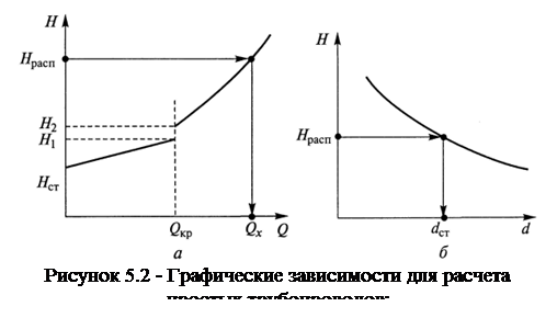
Having a characteristic of the required head for a given pipeline, it is possible, according to the known value of the available head H rasp find the required flow rate Q x (see figure 5.2, and).

If you need to find the inner diameter of the pipeline d, then, setting several values d, it is necessary to build the dependence of the required pressure H waste from diameter d (fig.5.2, b). Further by value N decthe nearest larger diameter is selected from the standard range d st .

In some cases, in practice, when calculating hydraulic systems, instead of the characteristic of the required head, the characteristic of the pipeline is used. Characteristics of the pipelineis the dependence of the total head losses in the pipeline on the flow rate. The analytical expression for this dependence is

Comparison of formulas (5.5) and (5.2) allows us to conclude that the characteristic of the pipeline differs from the characteristic of the required head by the absence of static head H st, and at H st = 0 these two dependencies coincide.

5.3 Simple piping connections.

Analytical and graphical calculation methods

Consider how to calculate the connections of simple pipelines.

Let we have serial connectiona few simple pipelines ( 1 , 2 and 3 in figure 5.3, and) different lengths, different diameters, with a different set of local resistances. Since these pipelines are connected in series, each of them has the same flow rate Q. The total head loss for the entire connection (between points Mand N) consists of the head loss in each simple pipeline ( , , ), i.e. for a serial connection, the following system of equations is valid:

(5.6)

The head loss in each simple pipeline can be determined through the values \u200b\u200bof the corresponding flow rates:

The system of equations (5.6), supplemented by dependencies (5.7), is the basis for the analytical calculation of a hydraulic system with a series connection of pipelines.

If a graphical calculation method is used, then it becomes necessary to build the total characteristics of the connection.

In Figure 5.3, b shows a method for obtaining the summation of the serial connection. For this, the characteristics of simple pipelines are used. 1 , 2 and 3

To construct a point belonging to the total characteristic of a series connection, it is necessary, in accordance with (5.6), to add the head losses in the original pipelines at the same flow rate. For this purpose, an arbitrary vertical line is drawn on the graph (at an arbitrary flow rate Q" ). Along this vertical, the segments (head losses, and) obtained from the intersection of the vertical with the original characteristics of the pipelines are summed up. The point thus obtained ANDwill belong to the total characteristic of the connection. Consequently, the total characteristic of a series connection of several simple pipelines is obtained by adding the ordinates of the points of the initial characteristics at a given flow rate.

Parallelis called the connection of pipelines that have two common points (branching point and closing point). An example of a parallel connection of three simple pipelines is shown in figure 5.3, in.Obviously, the consumption Q fluid in the hydraulic system before branching (point M)and after closing (point N) the same and equal to the amount of expenses Q 1 , Q 2 and Q 3 in parallel branches.

If we designate the full heads at the points M and Nthrough H M and H N, then for each pipeline the head loss is equal to the difference between these heads:

; ; ,

that is, in parallel pipelines, the head losses are always the same. This is due to the fact that with such a connection, despite the different hydraulic resistances of each simple pipeline, the costs Q 1 , Q 2 and Q 3 distributed between them so that the losses remain equal.

Thus, the system of equations for parallel connection has the form

(5.8)

The head loss in each pipeline entering the connection can be determined by formulas of the form (5.7). Thus, the system of equations (5.8), supplemented by formulas (5.7), is the basis for the analytical calculation of hydraulic systems with parallel connection of pipelines.

In Figure 5.3, r shows a method for obtaining a summary characteristic of a parallel connection. For this, the characteristics of simple pipelines are used. 1 , 2 and 3 , which are built according to dependencies (5.7).

To obtain a point belonging to the total characteristic of a parallel connection, it is necessary, in accordance with (5.8), to add up the flow rates in the original pipelines at the same head losses. For this purpose, an arbitrary horizontal line is drawn on the graph (with an arbitrary loss). Along this horizontal line, the segments (costs Q 1 , Q 2 and Q 3), resulting from the intersection of the horizontal line with the original characteristics of the pipelines. The point thus obtained INbelongs to the total characteristic of the connection. Consequently, the total characteristic of the parallel connection of pipelines is obtained by adding the abscissas of the points of the initial characteristics for given losses.

The summary characteristics for branched pipelines are constructed using a similar method. Branched connectionis a set of several pipelines having one common point (the place of branching or closing of pipes).

The series and parallel connections discussed above, strictly speaking, belong to the category of complex pipelines. However, in hydraulics under complex pipeline,as a rule, they understand the connection of several simple pipelines connected in series and in parallel.

In Figure 5.3, dan example of such a complex pipeline consisting of three pipelines is given 1 , 2 and 3. Pipeline 1 included in series with respect to pipelines 2 and 3. Pipelines 2 and 3 can be considered parallel, since they have a common branch point (point M) and supply fluid to the same hydraulic tank.

For complex pipelines, the calculation is usually carried out graphically. The following sequence is recommended:

1) a complex pipeline is split into a series of simple pipelines;

2) for each simple pipeline its characteristic is built;

3) by graphical addition, a characteristic of a complex pipeline is obtained.

In Figure 5.3, eshows a sequence of graphical constructions when obtaining a summary characteristic () of a complex pipeline. First, the characteristics of pipelines are added and according to the rule of adding characteristics of parallel pipelines, and then the characteristic of a parallel connection is added to the characteristic according to the rule of adding characteristics of series-connected pipelines and the characteristic of the entire complex pipeline is obtained.

Having a graph constructed in this way (see Figure 5.3, e) for a complex pipeline, it is possible quite simply by the known flow rate Q 1 entering the hydraulic system, determine the required head H cons \u003d for the entire complex pipeline, costs Q 2 and Q 3 in parallel branches, as well as head losses, and in each simple pipeline.

5.4 Pumped piping

As already noted, the main method of supplying liquid in mechanical engineering is forced pumping of it by a pump. By pumpis called a hydraulic device that converts the mechanical energy of the drive into the energy of the flow of the working fluid. In hydraulics, a pipeline in which the movement of fluid is provided by a pump is called pumped pipeline(Figure 5.4, and).

The purpose of calculating a pumped pipeline is usually to determine the head created by the pump (pump head). Pump head Н n is called the total mechanical energy transferred by the pump to a unit of fluid weight. Thus, to determine H n it is necessary to estimate the increment of the total specific energy of the liquid when it passes through the pump, i.e.

, (5.9)

where H in, H out -the specific energy of the liquid, respectively, at the inlet and outlet of the pump.

Consider the operation of an open pipeline with a pumping feed (see Figure 5.4, and). The pump is pumping liquid from the lower reservoir ANDwith pressure above the liquid p 0 to another tank B,in which pressure r 3 . Height of the pump location relative to the lower liquid level H 1 is called the suction head, and the pipeline through which the liquid enters the pump is suction pipe,or suction line. Height of the location of the final section of the pipeline or the upper liquid level H 2 is called the discharge head, and the pipeline through which the fluid moves from the pump is pressured,or hydraulic pressure line.

Let us write down the Bernoulli equation for the fluid flow in the suction pipeline, i.e. for sections 0-0 and 1-1 :

, (5.10)

where is the head loss in the suction pipeline.

Equation (5.10) is basic for calculating the suction pipelines. Pressure p 0 usually limited (most often atmospheric pressure). Therefore, the purpose of calculating the suction line is usually to determine the pressure upstream of the pump. It must be higher than the vapor pressure of the liquid. This is necessary to avoid the occurrence of cavitation at the pump inlet. From equation (5.10), you can find the specific energy of the fluid at the pump inlet:

. (5.11)

We write the Bernoulli equation for the fluid flow in the pressure pipeline, i.e., for the cross-sections 2-2 and 3-3:

, (5.12)

where is the pressure loss in the pressure pipeline.

The left side of this equation is the specific energy of the fluid at the pump outlet H out... Substituting in (5.9) the right-hand sides of dependencies (5.11) for H in and (5.12) for H out, we get

As follows from equation (5.13), the pump head H n provides liquid rise to a height (H 1+H 2), an increase in pressure with r 0 before p 3 and is spent on overcoming resistances in the suction and discharge pipelines.

If on the right-hand side of equation (5.13) designate H st and replace on the KQ m , then we get H n= H cr + KQ m.

Let's compare the last expression with the formula (5.2), which determines the required head for the pipeline. Their complete identity is obvious:

those. the pump generates a head equal to the required pipeline head.

The resulting equation (5.14) allows you to analytically determine the pump head. However, in most cases, the analytical method is rather complicated, therefore, a graphical method for calculating a pipeline with a pumping feed has become widespread.

This method consists of jointly plotting the characteristics of the required head of the pipeline (or characteristics of the pipeline) and pump characteristics. The pump characteristic is understood as the dependence of the head created by the pump on the flow rate. The intersection point of these dependencies is called operating pointhydraulic system and is the result of the graphical solution of equation (5.14).

Figure 5.4, ban example of such a graphical solution is given. Here point A is the desired operating point of the hydraulic system. Its coordinates determine the pressure H n generated by the pump and flow rate Q n fluid from the pump to the hydraulic system.

If, for some reason, the position of the operating point on the graph does not suit the designer, then this position can be changed by adjusting any parameters of the pipeline or pump.

7.5. Water hammer in the pipeline

Water hammeris called an oscillatory process that occurs in a pipeline with a sudden change in the fluid velocity, for example, when the flow stops due to the rapid shutdown of a gate valve (tap).

This process is very fast and is characterized by an alternation of a sharp increase and decrease in pressure, which can lead to the destruction of the hydraulic system. This is due to the fact that the kinetic energy of the moving flow, when stopped, turns into work to stretch the walls of the pipes and compress the fluid. The greatest danger is the initial pressure surge.

Let us trace the stages of the water hammer that occurs in the pipeline when the flow is quickly cut off (Figure 7.5).

Let at the end of the pipe, along which the liquid moves at a speed vq, the tap was instantly closed AND.Then (see figure 7.5, and) the velocity of the liquid particles hitting the tap will be extinguished, and their kinetic energy will go into the work of deformation of the pipe walls and the liquid. In this case, the pipe walls are stretched, and the liquid is compressed. The pressure in the stopped fluid increases by Δ p beats Other particles run into the decelerated liquid particles near the crane and also lose speed, as a result of which the cross section pnmoves to the right at a speed s called the speed of the shock wave,the transition region itself (section p-p),in which the pressure changes by the value Δ p oud, called shock wave.

When the shock wave reaches the reservoir, the liquid will be stopped and compressed throughout the pipe, and the pipe walls will be stretched. Shock pressure rise Δ p beats will spread to the entire pipe (see Fig. 7.5, b).

But this state is not equilibrium. Under the influence of increased pressure ( r 0 + Δ p beats) liquid particles will rush from the pipe into the reservoir, and this movement will begin from the section directly adjacent to the reservoir. Now the section pnmoves through the pipeline in the opposite direction - to the crane - at the same speed fromleaving a pressure in the liquid p 0 (see figure 7.5, in).

The fluid and pipe walls return to the initial state corresponding to the pressure p 0 . The work of deformation is completely converted into kinetic energy, and the liquid in the pipe acquires its initial velocity , but directed in the opposite direction.

At this speed, the "liquid column" (see figure 7.5, r) tends to break away from the tap, resulting in a negative shock wave (the pressure in the liquid decreases by the same value Δ p beats). The boundary between two fluid states is directed from tap to tank at speed from, leaving behind the compressed pipe walls and the expanded liquid (see figure 7.5, d). The kinetic energy of the fluid is again transferred to the work of deformation, but with the opposite sign.

The state of the liquid in the pipe at the time of the arrival of a negative shock wave to the reservoir is shown in Figure 7.5, e.As in the case shown in Figure 7.5, b, it is not in equilibrium, since the liquid in the pipe is under pressure ( r 0 + Δ p beats), less than in the tank. In figure 7.5, fshows the process of equalizing the pressure in the pipe and the tank, accompanied by the occurrence of fluid movement at a speed .

Obviously, as soon as the shock wave reflected from the tank reaches the valve, a situation will arise that already took place at the moment of closing the valve. The entire water hammer cycle will be repeated.

The theoretical and experimental studies of hydraulic shock in pipes were first performed by N.E. Zhukovsky. In his experiments, up to 12 complete cycles were recorded with a gradual decrease in Δ p beats As a result of his studies, N.E. Zhukovsky obtained analytical dependences that allow estimating the shock pressure Δ p beats One of these formulas, named after N.E. Zhukovsky, has the form

where the velocity of propagation of the shock wave fromdetermined by the formula

,

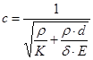where K -bulk modulus of elasticity of the liquid; E -modulus of elasticity of the pipeline wall material; d and δ are the inner diameter and wall thickness of the pipeline, respectively.

Formula (7.14) is valid for direct water hammer, when the flow cutoff time t close is less than the water hammer phase t 0:

where l - pipe length.

Water hammer phase t 0 is the time it takes for the shock wave to travel from the tap to the tank and back. When t closed\u003e t 0, the shock pressure is less, and such a water hammer is called indirect.

If necessary, you can use the known methods of "mitigating" water hammer. The most effective of these is to increase the response time of taps or other devices that shut off the fluid flow. A similar effect is achieved by installing accumulators or safety valves in front of devices that block the flow of liquid. A decrease in the velocity of fluid movement in a pipeline due to an increase in the inner diameter of pipes at a given flow rate and a decrease in the length of pipelines (a decrease in the water hammer phase) also contribute to a decrease in shock pressure.

[Table of contents] [Next lecture] VIP-user.
This can be done completely free of charge. Read on.

The most likely causes of irregularities in the operation of the water supply system in a private house are, as you know, corrosion of pipe walls, salt deposition on them and high water pressure in the pipeline. Taking into account the fact that in recent years to replace metal pipes more and more often their plastic counterparts come, only the last two of the reasons listed above pose a real threat to your water supply. The issue of combating salt deposits does not fall within the scope of our article (although they partially affect the pressure indicators in the pipes), in connection with which we will only consider the last factor.

For warning possible problems before buying pipe products, you must familiarize yourself with the passport attached to them and make sure that they are able to withstand the pressures provided for in your water supply system.

Note! Increased pressure in the system leads to an increase in water consumption.

This leads to additional consumption of electricity consumed by the pumping equipment, which ensures continuous circulation of water in the system.

Pressure value

It is well known that maintaining a normal level of water pressure in pipes is the most important condition for the operability of the water supply network, as well as for its long-term and trouble-free operation. At the same time, the value of pressure in the pipeline may differ significantly from the fixed average indicator, standardized for domestic water supply systems.

So, for example, for the normal operation of a kitchen valve, the carrier pressure in the water supply system should not be less than 0.5 bar.

But in real conditions, the value of this indicator, as a rule, slightly differs from the indicated value. That is why, when accepting the water supply system (after its repair, in particular), it is advisable to check the working pressure for compliance with the established standards.

Well, in the case of independent laying of pipelines, before starting work, you should carefully read the basic requirements for household water supply systems, as well as the generally accepted procedure for their arrangement.

Pressure equalization devices

Let's look at some tools to help equalize the pressure.

To equalize the water pressure in household pipelines, special devices can be used to remove excess media. Moreover, the excess pressure in the system can be compensated very simply - for this, a so-called expansion tank is installed in it, which takes over all the surplus of the carrier.

In accordance with their design, all known samples of expansion (compensation) tanks are divided into open and closed devices. They are very often used in facility supply systems. hot water, since in this case the probability of the formation of pressure drops in the system is very high. This is due to the fact that the coolant in the course of its circulation through the network (from the "return" to the heating boiler, and then back to the system) somewhat increases its volume.

Note! When the water temperature changes by 10 ° C, for example, the expansion rate of the coolant in the system reaches 0.3% of the total volume of liquid in it.

The disadvantage of open-type expansion devices is that their installation translates the system into a mode characterized by low coolant pressure and, as a result, poor controllability. In addition, a gradual evaporation of the carrier occurs in an open system. It will take extra effort on your part to restore it continuously.

To all of the above, you can add the fact that, due to the openness of the tank, fresh portions of air constantly enter it, which causes acceleration of corrosive processes in the system.

Note! Since open-type expansion tanks must be located at the very top of the structure, they require mandatory insulation. It is clear that the cost of the entire water supply system as a whole in this case increases significantly.

All the above troubles can be avoided by using a closed-type tank as a compensating device, the installation location of which, as a rule, is not standardized. These tanks are equipped with a built-in membrane mechanism that allows you to regulate the pressure of the carrier in closed mode.

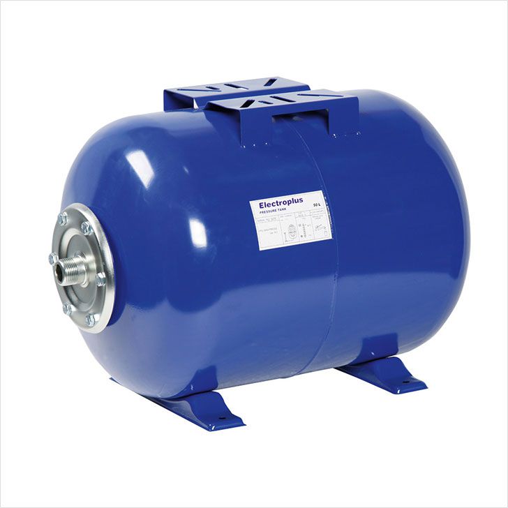
In addition to compensation tanks, so-called hydraulic accumulators can also be installed in water supply systems, used to protect the pipeline from such a dangerous phenomenon as water hammer.

The phenomenon of water hammer usually manifests itself when the pumping equipment is disconnected from the network or when the water intake valve is suddenly closed (opened). The resulting dynamic loads can significantly exceed the values \u200b\u200bpermissible for a particular pipeline. Note that such devices are used, as a rule, in pipelines with drinking water and allow you to create a small supply of the carrier, which can be automatically redirected back to the system (in case of pressure drop in it).
Like the previously considered compensation devices, accumulators can be made in a closed or open form and have all the disadvantages listed above.

Note! Simultaneously with hydraulic accumulators, it is recommended to place small expansion tanks (about 0.2 liters) at the points of water intake.

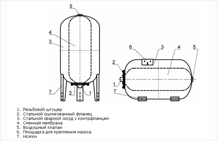
When studying the design of the simplest closed-type hydraulic accumulator, we find that its action is based on the same membrane mechanism (similar to an expansion tank). In a closed volume, the membrane is in a stable state, balanced by approximately equal pressures of the coolant and the air bubble, located on opposite sides of the partition.
After turning on the pumping station, the volume of the coolant in the system increases, which leads to the compression of air in the membrane cylinder and, as a result, an increase in its pressure. This change is automatically transmitted to the sensitive element of the built-in relay, which turns off the pump when this parameter reaches a certain value.

In the process of consuming water in the system, its pressure decreases noticeably, which again leads to the operation of the relay, but now to turn on.
Hydraulic performance

Calculation of the carrier pressure sufficient for the normal functioning of your water main will allow you to accurately determine the samples of pipe products purchased before its installation. It should be remembered that the limit values \u200b\u200bof pressure in the network are usually associated with the following indicators:

• upper and lower fluid pressure thresholds, which are designed for closed-type compensating devices installed in the network (expansion tank and hydraulic accumulator);
• pressure values \u200b\u200bthat create conditions for the normal functioning of household appliances, dependent on water supply (washing machine, for example);
• the limiting pressure values \u200b\u200bfor which the pipes you purchased and the accessories supplied with them (valves, tees, mixers, etc.) are designed.

Note! The unit of measurement of the pressure of the carrier circulating in the water supply networks is 1 bar (or 1 atmosphere). The value of this indicator for city water mains (according to the requirements of the current SNiP) should be about 4 atmospheres.

We also note that the valves, mixers installed in the heating pipeline, as well as the pipes themselves must withstand short-term pressure surges up to 6 atmospheres. When buying basic household equipment connected to your water supply network, you should choose models that have a small margin of safety in terms of the ultimate indicator. Such foresight will allow you to protect them from sudden pressure surges in the network caused by hydraulic shocks.

At the same time, it is very important that the water pressure in the water supply system of a private house has a level that allows several consumption points to be simultaneously turned on at once, which can be ensured with a minimum indicator of 1.5 bar.

For direct reading of pressure in the water supply network, standard measuring manometers with a standard linear scale are used, calibrated in the appropriate units.

According to the requirements of SNiP, the operability of devices in the heating network, as well as the condition of all auxiliary equipment, should be checked at least once a year.

During this check, first of all, the presence of leaks in the water supply system and the pressure drop caused by them are established. After all leaks are eliminated, it will be necessary to check the pressure in the water supply system according to the pressure gauge installed on the main hydraulic accumulator.

During normal operation of the system, the reading of this device should be close to the minimum value (Pmin). If there is a noticeable difference from Pmin (more than 10%), you will need to try to increase the pressure to the desired value by turning on the pumping equipment operating in your network. When the water pressure in the heating network increases (immediately after the pump stop relay has triggered), it will be necessary to measure the pressure again, but now in the shutdown mode. The specified parameter, by analogy with the previous case, should not differ from the Pmax value by more than 10%.

Introduction

Goals and objectives of the course work

1. Calculation of the pipeline

1.1 Quest

1.2 Calculations

1.2.1 Determination of speeds and costs

1.2.2 Determination of static and velocity head

1.2.3 Calculation of head losses

1.2.4 Determining the required head

2. Selection of the pump

3. Pump regulation

4. Calculation of the permissible suction lift

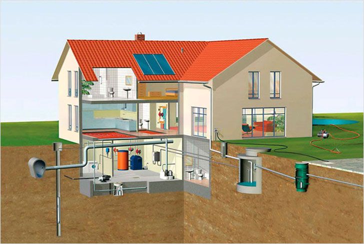
Technological pipelines are such pipelines of industrial enterprises, through which mixtures, intermediates and finished products, spent reagents, water, fuel, and other materials are transported, which ensure the conduct of the technological process.

With the help of technological pipelines at chemical enterprises, products are moved both between individual devices within the same workshop or technological unit, and between technological units and separate workshops, feed raw materials from storage facilities or transport finished products to the place of their storage.

In the chemical industry, process pipelines are an integral part of the process equipment. The costs of their construction in some cases can reach 30% of the cost of the entire enterprise. In some chemical plants, the length of pipelines is measured in tens or even hundreds of kilometers. Uninterrupted operation of technological units and a chemical enterprise as a whole, the quality of products and safe operating conditions of technological equipment largely depend on how well the pipelines are designed and operated, and at what level their good condition is maintained.

Raw materials and products used in chemical technology and transported through pipelines have different physical and chemical properties. They can be in a liquid, plastic, gas or vapor state, in the form of emulsions, suspensions, or carbonated liquids. The temperatures of these media can be in the range from low minus to extremely high, pressure - from deep vacuum to tens of atmospheres. These media can be neutral, acidic, alkaline, flammable and explosive, hazardous to health and environmentally hazardous.

Pipelines are divided into simple and complex, short and long. Pipelines that do not have branches along the path of the liquid in the pipe for withdrawing or additional supply of liquid to the pipeline are called simple. Complex pipelines include pipelines consisting of a main trunk pipe and side branches that form a network of pipelines of various configurations. Most of the pipelines for technological installations of chemical enterprises are simple.

The simplest way to move liquid from one apparatus to another is to drain it by gravity. Such movement is possible only if the initial container is located above the filled one.

· Acquaintance with the device of technological pipelines of chemical enterprises, methods of moving liquids through them and methods of using fundamental dependencies to obtain the design equations necessary for constructing the hydraulic characteristics of pipelines.

Implementation of an individual task to build a curve of the required head for simple process pipeline, determining the method of moving fluid along it for a given flow rate, and selecting a pump, as well as acquiring the skill of analyzing the operation of a pipeline based on its hydraulic characteristics.

1.1 Assignment for term paper number 1 in the discipline "Processes and devices of chemical technology"

Option I-1

Perform hydraulic calculation of the process pipeline and build the required pressure curve. Select a pump for pumping liquid through the pipeline at a given flow rate.

Piping diagram

Calculation data:

RA \u003d 1.5 kg / cm2 h; PB \u003d 0.5 kg / cm2 vac; L1 \u003d 200 m; L2 \u003d 150 m; d1 \u003d 95x5 mm; d2 \u003d 45x4 mm;

The pumped-over liquid: Sulfuric acid 60%;

Local resistance type: 1-valve normal;

2-branch φ \u003d 90 °;

Type and condition of the pipe: 1-steel with large deposits;

2-steel new;

Sudden change in diameter: sudden narrowing

Lift height of liquid: ΔZ \u003d 40 m;

The flow rate of the pumped-over liquid: qv \u003d 1.8 · 10-3 m3 / s.

We translate, where necessary, the initial data into the SI system:

For 60% sulfuric acid, the reference values \u200b\u200bfor density and dynamic viscosity are, respectively: ,Pass;

Let's set 6 values \u200b\u200bof the velocity in the section of the pipe with a smaller diameter (II section of the pipeline) from the interval m / s.

Let's find the volumetric flow rate of the liquid:

qv1 \u003d 5.37 10-4 m3 / s;

qv2 \u003d 1.07 10-3 m3 / s;

qv3 \u003d 1.61 10-3 m3 / s;

qv4 \u003d 2.15 10-3 m3 / s;

qv5 \u003d 2.69 10-3 m3 / s;

qv6 \u003d 3.22 10-3 m3 / s;

Let's calculate the cross-sectional area of \u200b\u200bthe first pipe:

Let's find the speed of the fluid flow in the first pipe:

We get: uI, 1 \u003d 0.10 m / s;

uI, 2 \u003d 0.19 m / s;

uI, 3 \u003d 0.28 m / s;

uI, 4 \u003d 0.38 m / s;

uI, 5 \u003d 0.47 m / s;

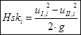
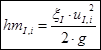
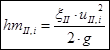
The head required to overcome the resistance of the liquid column:

where .

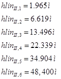
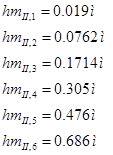
Velocity head:

Let's calculate the pressure loss:

To do this, we find the values \u200b\u200bof the Reynolds criterion for the liquid in the first pipe:

Roughness pipes :

For the first steel pipe with large deposits we take

Then

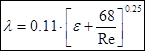
Since all values \u200b\u200bof the Reynolds criterion are included in the interval, then for a mixed turbulent flow, the following formula can be used to calculate the friction coefficient:

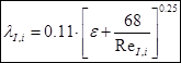
Then the losses in the 1st linear section of the pipeline will be equal:

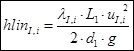
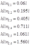
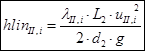
Losses in the 2nd linear pipe section:

Pipe roughness:

For the second new steel pipe we will take: m.

Then:

Reynolds criterion critical values:

Since the first 4 values \u200b\u200bof the Reynolds criterion are less than ReКР1, the flow is smooth turbulent, and:

We get:

Since the last two values \u200b\u200bof Re belong to the interval, the flow is mixed turbulent, and:

then

Head loss in the second section of the pipeline:

, we find:

Let's find the pressure loss in local resistances.

To do this, we select the reference values \u200b\u200bof the coefficients of local losses for the corresponding local resistances:

The entrance to the pipe;

The valve is normal;

Sudden narrowing;

Bend φ \u003d 90 °;

Exit from the pipe;

Then for Ipipe:

For II pipe:

Local losses in the I section:

, we get:

Local losses in section II:

Then the total losses in the I and II sections:

In the 1st section:

On the 2nd section:

Total losses:

We find the value of the actual head:

We find the required pressure:

Based on the calculations performed, we will construct the curve of the required pressure.

In this work, the selection of a pump consists in finding a pump for which the operating point, when combined with the curve of the required pressure, was located within the pump area, and for which the usual flow rate qv was equal to the flow rate set for the pipeline or differed from it in a larger direction. In this case, the excess flow rate can be repaid by closing the shut-off device.

With the help of a pump to ensure a liquid flow rate of m3 / s \u003d m3 / h, it is necessary to create the required head Hreq \u003d 38m.

We will select a pump to ensure such conditions:

Let's define the working area for the required liquid flow rate:

m3 / s;

m3 / s.

Let's find the heads corresponding to such costs:

From the ratio, substituting H1 \u003d 24 m, qv1 \u003d 2.4 10-3 m3 / s and, accordingly, m3 / s and m3 / s we find m; m.

Using the three available points, we will construct the pump curve.

It can be seen that the curve of the required head and the pump intersect practically in the working area. In addition, the pump provides a small additional margin for flow and head. To increase the required pressure in the network, it is necessary to use a shut-off and control device (valve). When it is partially blocked, the flow cross section decreases and the local resistance value increases, which leads to a counterclockwise displacement of the pressure curve.

The method of regulating the pump flow by changing the number of shaft revolutions is the most effective from the standpoint of saving energy resources. At the same time, relatively cheap, reliable and easy-to-use asynchronous electric motors are often used to drive pumps. Changing the speed of such motors is associated with the need to change the frequency of the supply AC. This method turns out to be complex and costly. In this regard, throttling is mainly used to regulate the pump flow.

A change in the position of the valve flywheel is accompanied by a change in the coefficient of local resistance. If the change in speed is an effect on the pump characteristic, then throttling is a change in the network characteristic.

If, for example, you close the valve, thereby increasing the pressure loss in the network, as can be seen from the equation for calculating the local pressure loss, an increase in the local resistance coefficient will lead to an increase in the pressure loss. Accordingly, the required head will also increase. The new characteristic of the network will be steeper. In this case, the operating point will shift towards lower costs.

Let us calculate the net power expended by the pump to communicate pressure energy to the fluid:

Shaft power (taking into account pump efficiency): kW;

The power consumed by the motor (nominal), taking into account the fact that the transmission efficiency is equal to one: kW;

Taking the power reserve factor, we find the installed engine power:

Considering that the rated power of the selected pump is slightly higher than the calculated one, it allows us to conclude that the most suitable pump is selected.

Bypass (bypass). When regulating the pump flow in this way, the required liquid flow rate in the system is ensured by diverting a part of the liquid pumped by the pump from the pressure pipeline to the suction pipeline through the bypass pipeline. If it is necessary to reduce the flow to the system, open the valve on the bypass line. The characteristic of the network will become flatter and the total pump flow increases.

This method of regulation is more economical for pumps in which the power consumption decreases with increasing flow. On centrifugal pumps, bypass control will increase pump power and may overload the motor.

Bypassed from the pressure side to the suction side, the fluid flow has some energy. If, during regulation by bypass, there is no useful transfer of energy from the bypass fluid to the flow suitable for the impeller, the power loss can be determined by the formula:

,

where qН - pump flow,

qП - by-pass flow,

Nset is the power consumed by the pumping unit.

Then kW.

The energy of the bypass flow can be efficiently used in two ways:

1) To increase the pressure in the suction cavity of the pump by creating an ejection effect by the bypass flow; sequentially to the main pump, the water-jet pump is switched on, removing part of the surmountable head from the main pump, so that the main pump operates at a lower head and improved cavitation conditions.

2) For swirling the flow in front of the impeller. Swirling of the flow is carried out in the direction of rotation of the impeller, while there is a pseudo-decrease in the frequency of rotation of the impeller n to the frequency of rotation of the swirling fluid flow. Pump parameters - head, flow rate and power consumption will change.

When designing a pumping system, a check is made to ensure the permissible suction lift.

The reason for this is that the head (and most often the pressure) at the inlet to the suction line is higher than at the inlet to the pump by the amount of losses in the suction line. Typically, the pump inlet pressure is below atmospheric (vacuum). The magnitude of the vacuum, in turn, is limited by the magnitude of the atmospheric pressure.

When the vapor pressure is reached, the liquid begins to boil. The higher the temperature, the higher the saturated vapor pressure. Steam entering the pump disrupts its operation. In dynamic pumps, the generated pressure depends on the density of the liquid. Steam has a density almost 1000 times less than that of a liquid. The pressure drops accordingly. In positive displacement pumps, the flow rate also decreases due to the low vapor density, and leakage through leaks increases.

Another phenomenon that is extremely undesirable during pump operation and caused by a decrease in suction pressure is cavitation (boiling of a liquid in a zone of reduced pressure (for example, behind the edge of the pump blades), followed by the collapse of the formed bubbles in the zone of pressure increase). When the vapor bubble collapses, the liquid moves to its center. In this case, the liquid acquires a certain speed. In the center of the vapor cavity, the liquid stops instantly, because the liquid is practically incompressible. Kinetic energy turns into potential energy (pressure increase). The fluid pressures are so great that destruction of the blade metal occurs in the cavitation zone.

In this regard, the calculation is made based on the condition of the pump without cavitation. In practice, one more quantity has to be taken into account - the so-called cavitation reserve.

The permissible suction lift depends on the vapor pressure. The closer the liquid temperature is to the boiling point, the higher the saturated vapor pressure, and, therefore, the pump can be raised to a lower height relative to the liquid surface. Even a negative value can be obtained as a result of calculations. Indeed, when pumping low-boiling liquids, the pumps have to be buried (installed below the surface of the liquid).

The fluid velocity also reduces the allowable suction lift due to the velocity head and head loss in the suction line. In this regard, when designing pumping units, they try to make the diameters of the suction pipelines large. Any local resistance is also highly undesirable. Various kinds of filters, valves or valves, if possible, are installed not on the suction, but on the discharge pipeline.

Thus:

where:

Pt \u003d 200 mm Hg \u003d 26.66 103 Pa - saturated steam pressure

sulfuric acid at operating temperature (25 ° C);

UBC \u003d\u003d m / s - the speed of the liquid in the suction pipe of the pump;

Let us find hPOT - head loss in the suction line:

The flow is mixed turbulent, therefore:

m - cavitation reserve.

· P1 \u003d 1.472 · 105 Pa - pressure in the suction pipeline.

conclusions

In this work, the calculation of the technological pipeline (determination of the required pressure) was carried out, consisting of the determination of the static, velocity head, as well as local and linear resistances on different sites and throughout the pipeline as a whole. The curve of the required pressure was built, and the selection of the pump was made, which provides the flow rate of the transported liquid specified by the teacher.

1. A.G. Kasatkin, "Basic processes and devices of chemical technology", Moscow: Chemistry, 1971 - 784 p.

2. The main processes and devices of chemical technology: Design manual / GS. Borisov, V.P. Brykov, Yu.I. Dytnersky et al. Ed. Yu.I. Dytnersky, 2nd ed., Revised. and add. Moscow: Chemistry, 1991 - 496 p.

3. K.F. Pavlov, P.G. Romankov, A.A. Noskov. Examples and tasks for the course of chemical processes and devices. technologies, 10th ed., rev. and add. Ed. P.G. Romankov. L .: Chemistry, 1987 - 578 p.